Non-Collapsible State Separation — v3.7 (Current)

Current version, June 2026. Adds Theorem 3 (Orthogonal Defense Layers), Corollary 3.1 (Nilpotency), Proposition 1.4, and Open Problems 7–10. This is the flagship proof document.

Non-Collapsible State Separation

as a Structural Solution to Signal Smearing in Adaptive State Estimation Systems

Gregory Stuart Lacefield · Independent Researcher · Lacefield Research · Las Vegas, NV

gregorylacefield.com · Preliminary Draft · May 2026 · Provisional Patent Filed June 2026

Abstract

We model adaptive state estimation systems as structural causal models over four categorically distinct signal classes: environmental context (S), genuine internal state (D), interface friction (I), and execution output (C). Standard architectures collapse these classes into a single composite measurement, making it impossible to recover D from observed output by statistical means alone. We prove that enforcing a strictly lower-triangular causal pipeline with non-collapsible profiles eliminates reverse-path causal influence from execution state to internal state. We further prove that a prerequisite-gated update rule combined with a circuit-breaker protocol preserves the integrity of confirmed internal state during execution anomalies. Both results are domain-independent and follow from graph topology rather than distributional assumptions. The architecture has been instantiated in education, industrial operations, athletic training, and autonomous vehicle monitoring.

Contributions

This paper makes the following contributions:

• Formalizes the signal smearing problem as a structural (rather than statistical) failure in adaptive state estimation systems.

• Proves that a strictly lower-triangular causal pipeline with non-collapsible profiles eliminates reverse-path causal influence from execution state to internal state (Theorem 1).

• Proves that a prerequisite-gated update rule combined with a circuit-breaker protocol preserves schema floor integrity during execution anomalies (Theorem 2).

• Establishes that both results are domain-independent and depend only on graph topology.

• Provides a clear architectural distinction between structural guarantees and post-hoc statistical correction methods used in prior work.

• Specifies the enforcement requirements needed to realize these guarantees in practice.

1. The Signal Smearing Problem

Adaptive systems that monitor a human operator or learner and adjust their behavior in response must solve a diagnostic problem: given observed output Y, what is the current genuine internal state of the human? This question cannot be answered by any system whose measurement architecture collapses the genuine internal state with environmental noise, interface friction, and physical execution variance onto a single channel. We formalize this failure and prove it is structural.

Definition 1.1 (Signal Classes).

Let the state of a human-system interaction be characterized by four categorically distinct random variables:S — Environmental state. Ambient conditions and system-side noise acting on the human.D — Internal state. The human’s genuine internal understanding or capacity. This is the target of inference.I — Interface state. Presentation and delivery variables imposed by the system.C — Execution state. Raw physical and neuro-motor performance signals.The four variables S, D, I, C are generated by categorically distinct physical and cognitive mechanisms and are therefore causally independent at source.

Definition 1.2 (Smeared Architecture).

A standard adaptive system observes a composite measurement M = f(S, D, I, C), where f is a function that combines all four signal classes onto a single output channel. In this architecture, the partial derivatives ∂M/∂D and ∂M/∂C are not identically zero and are coupled through the shared channel.

Proposition 1.3 (Non-Recoverability of Smeared Signals).

Let M be generated by a smeared architecture. Then for any measurable function g, the estimator D̂ = g(M) satisfies E[‖D̂ − D‖²] > 0 if Var(C) > 0 and the channel function f is not invertible in D given C.

Proof.

Since M = f(S, D, I, C) and C contributes non-trivially to M (Var(C) > 0), any estimator g(M) conflates variation in D with variation in C. Because f is not assumed invertible in D given C, the information required to separate these contributions is not present in M. The mean squared error of any estimator D̂ = g(M) is therefore bounded away from zero.

■

Remark 1.4. Proposition 1.3 establishes that the smearing problem is not a statistical estimation problem amenable to better algorithms. It is a structural information problem: the data required to separate D from C is not present in M because it was never recorded separately. This motivates the architectural intervention of Section 2 rather than a refined estimator.

Empirical confirmation (Test 5, Lacefield 2026b). Under identical coupling conditions (ε = 0.8, sustained), the smeared architecture produces corr(D_smeared, S) = 0.09–0.14 across three coupling schedules, while the NCFCA architecture produces corr(D_protected, S) ≈ −0.0007 — a 200-fold reduction in S contamination of D. The smeared architecture cannot eliminate this contamination by any downstream statistical method, consistent with Proposition 1.3. (NCFCA Empirical Validation Suite, Test 5, Lacefield 2026b.)

Proposition 1.4 (Institutional Corruption Decay — Functional-Analytic Formulation).

Let Ω denote the state space of the adaptive system. Let A_t : Ω → ℝⁿ be a time-indexed observation mapping satisfying rank(A_t) < dim(Ω), and let ℱ be a closed estimator governed by the state update:ℱ_{t+1} = Φ(ℱ_t, A_t(Χ_t + Δ_t))where Χ_t ∈ Ω is the true state and Δ_t ∈ Ω is a persistent perturbation. If the estimator minimizes internal inconsistency by driving a coherence loss υ(ℱ_t) → 0, then for any Δ ∈ Ker(A_t), the estimator converges to a fixed point ℱ* = Χ* + Δ in which Δ is observationally indistinguishable from the true state.

Remark 1.5 (Data Processing Inequality as Non-Recoverability Proof). The non-recoverability of smeared signals follows directly from the Data Processing Inequality (Cover & Thomas, 2006). For any downstream estimator D̂ = g(M), the composite M = f(S, D, I, C) defines a Markov chain D → M → D̂. By the DPI: I(D; D̂) ≤ I(D; M). The inequality I(D; M) < H(D) holds strictly whenever the mixing function f is non-injective with respect to D — that is, whenever there exist distinct values of D that produce the same M given fixed S, I, C. This is the generic case under channel collapse: because M compresses four independent signal classes into one composite, different D values are aliased against different C, S, and I values, and the function f cannot be inverted to recover D. Therefore I(D; D̂) < H(D) for every possible estimator D̂ = g(M) — no processing of the smeared composite can achieve zero uncertainty about D. This is the information-theoretic proof of Proposition 1.3, requiring no assumptions about estimator bias or differentiability. The NCFCA breaks the smearing step by maintaining D in a separate write-protected data structure, preserving I(D; DSP) = H(D) by construction.

Remark 1.6 (Mutual Information Formalization of Signal Smearing). Signal smearing is formally the reduction of I(D; M) below H(D) caused by entanglement of D with independent signal classes S, C, and I in the composite M. In an unsmeared architecture, I(D; DSP) = H(D): the internal state channel carries maximal information about D because it receives only D-class signals. In a smeared architecture, H(D ∣ M) > 0 because M contains variation attributable to C, S, and I that cannot be distinguished from variation in D. The NCFCA non-collapsibility rule (Definition 2.2) is the architectural enforcement of I(D; DSP) = H(D): by prohibiting write paths from other signal classes into the DSP, the architecture guarantees that the DSP carries uncontaminated information about D. The information-theoretic grounding of diagnostic channel capacity limitations at scale is developed in Open Problem 7.

Remark 1.7 (Control Theory / Observability Framing of Non-Recoverability). The non-recoverability result of Proposition 1.3 can be restated in the language of observability from control theory (Kalman, 1960). A state D is observable from a measurement M if there exists a finite sequence of measurements that uniquely determines D. In the smeared architecture, the measurement M = f(S, D, I, C) defines an observation operator whose rank is strictly less than the dimension of the full state space (S, D, I, C). The component D lies in the unobservable subspace of this operator: different values of D produce identical M values when combined with appropriately different values of C, S, or I. By the Kalman observability rank condition, D is not observable from M. This means no linear or nonlinear observer — including Kalman filters, particle filters, and extended Kalman filters — can recover D with zero error from the composite measurement M. The NCFCA resolves this by constructing the system so that D is directly observable from its own dedicated channel (the DSP), not from a shared composite. This eliminates the observability defect entirely rather than working around it with more sophisticated estimators.

Remark 1.8 (Breakdown Point Theory and Architectural Contamination Resistance). The resistance of the NCFCA to execution-layer contamination can be characterized using the breakdown point framework of robust statistics (Huber, 1981). The breakdown point of an estimator is the maximum fraction of contaminated observations the estimator can tolerate before its output becomes arbitrarily bad. For any estimator D̂ = g(M) operating on a smeared composite M = f(S, D, I, C), the breakdown point with respect to C-channel contamination is 0: even a single observation where C deviates anomalously will affect M, and there is no estimator that can perfectly isolate D from C-induced variation in M when f is not invertible with respect to D. The NCFCA architecture achieves breakdown point 1 with respect to C-channel contamination of the DSP during anomaly windows: the circuit breaker protocol suspends all writes to the DSP, so 100% of anomalous C observations during the window have zero effect on the DSP record. This is not an improvement in estimator robustness — it is the elimination of the contamination pathway at the architectural level.

Remark 1.9 (Distributionally Robust Perspective on Non-Recoverability). The non-recoverability of smeared signals can be strengthened to a distributionally robust statement that holds without assuming a known data-generating distribution. Let ℙ be an ambiguity set of possible joint distributions over (S, D, I, C) — for example, all distributions within a given divergence ball around a nominal distribution, or all distributions consistent with observed first and second moments. For any estimator D̂ = g(M) operating on a smeared composite M = f(S, D, I, C), there exists a non-empty ambiguity set ℙ such that: sup_{P ∈ ℙ} ᵓc_P[L(D, D̂)] > 0 for any reasonable loss function L (squared error, 0-1 loss, or any strictly proper scoring rule). This holds because the mixing operation aliases distinct values of D against distinct values of C, S, and I, creating distributional overlap in M that no fixed estimator can eliminate across all distributions in ℙ. This is a strictly stronger statement than Proposition 1.3, which requires fixed distribution assumptions. The NCFCA architectural separation eliminates the aliasing at the data structure level, making the worst-case risk over ℙ zero for the DSP channel by construction — not by finding a robust estimator, but by removing the shared observation that creates distributional ambiguity.

Empirical confirmation, Propositions 1.3 and 1.4 (Test T0.3, Lacefield 2026b). The non-recoverability of smeared signals was stress-tested across seven coupling strengths (0.1 to 5.0) with 2,000 samples per condition. The NCFCA maintains constant MSE of 0.0026 across all coupling strengths because D is measured directly from its own channel, independent of C. The smeared best linear estimator's MSE grows from 0.129 at coupling 0.1 to 0.961 at coupling 5.0. The ratio of smeared MSE to NCFCA MSE grows from 49.5× at coupling 0.1 to 367.9× at coupling 5.0, monotonically. A cheating estimator that observes S and I (but not C) still cannot recover D: its MSE at coupling 2.0 is 4.003, which is 1,539× the NCFCA MSE. The irreducible error from C contamination grows without bound as coupling strength increases. The NCFCA MSE of 0.0026 is attributable solely to measurement noise and is independent of coupling strength. These results confirm Proposition 1.3 (estimator-theoretic bound), Proposition 1.4 (functional-analytic rank deficiency), Remark 1.5 (Data Processing Inequality), and Remark 1.9 (distributionally robust worst-case bound): no estimator operating on the smeared composite approaches the NCFCA’s accuracy regardless of coupling magnitude. (NCFCA Phase 0 Validation Suite, Test T0.3, Lacefield 2026b.)

2. The Non-Collapsible Four-Channel Architecture

We model the system as a structural causal model (V, G, F, Pᵤ) in the sense of Pearl (2000, Chapter 1). The distribution P over V is Markov with respect to G by construction. No faithfulness assumption is required; the interventional results that follow are identified by graph surgery on G without faithfulness.

Definition 2.1 (NCFCA Profiles).

The Non-Collapsible Four-Channel Architecture (NCFCA) maintains four independent profile structures:Sₛₒₚ — State Context Profile. Captures environmental state S. Resolved prior to any inference over D.Dᴅᴸᴾ — Dynamic State Profile. Captures internal state D. A directed acyclic graph of concept or skill nodes with mastery states. Write access subject to circuit-breaker suspension.Iᴵᴼᴾ — Interface Response Profile. Captures interface state I. Updated from Sₛₒₚ signals only.Cᴄᴇᴾ — Calibration Execution Profile. Captures execution state C. Acts as system circuit breaker.

Definition 2.2 (Non-Collapsibility Rule).

The four profiles Sₛₒₚ, Dᴅᴸᴾ, Iᴵᴼᴾ, Cᴄᴇᴾ must be maintained as structurally independent data structures. There shall exist no write path in the underlying data model that permits a value originating in Cᴄᴇᴾ (or Iᴵᴼᴾ) to directly modify any value stored in Dᴅᴸᴾ. The profiles may not be averaged, merged, or projected into a shared representation at any stage of processing or storage. All information flow between profiles must be unidirectional and must respect the lower-triangular causal order defined in Definition 2.3.Nomenclature equivalence: Throughout this proof, the four profiles Sₛₒₚ, Dᴅᴸᴾ, Iᴵᴼᴾ, Cᴄᴇᴾ are referred to by their signal class shorthand S, D, I, C respectively when the context is the causal signal rather than the data structure. The two notations are interchangeable: S ≡ Sₛₒₚ, D ≡ Dᴅᴸᴾ, I ≡ Iᴵᴼᴾ, C ≡ Cᴄᴇᴾ. Patent documents, technical specifications, and empirical reports in the NCFCA series use the same four designations. The signal class notation (S, D, I, C) is used in mathematical expressions and proofs; the profile notation (Sₛₒₚ, Dᴅᴸᴾ, Iᴵᴼᴾ, Cᴄᴇᴾ) is used when referring to the data structure implementation.

Remark 2.1 (Enforcement Mechanism). Enforcing the Non-Collapsibility Rule at the data-model level (rather than solely in application code) produces a structural guarantee analogous to a physical circuit breaker: the forbidden reverse-path influence cannot occur even if application logic contains errors or is later modified.

Definition 2.3 (Lower-Triangular Causal Pipeline).

Define the causal graph G over nodes {Sₛₒₚ, Dᴅᴸᴾ, Iᴵᴼᴾ, Cᴄᴇᴾ} with directed edges contained in:Eᴳ ⊆ { (Sₛₒₚ → Dᴅᴸᴾ), (Sₛₒₚ → Iᴵᴼᴾ), (Dᴅᴸᴾ → Cᴄᴇᴾ), (Iᴵᴼᴾ → Cᴄᴇᴾ) }The adjacency matrix of G is strictly lower-triangular under the ordering Sₛₒₚ ≺ Dᴅᴸᴾ ≺ Iᴵᴼᴾ ≺ Cᴄᴇᴾ.

Definition 2.4 (Circuit Breaker Protocol).

Let δ(t) be an anomaly indicator for the execution profile at time t. The write-suspension protocol is given by Φ(t) = 1 − δ(t), where Φ(t) = 1 permits writes to Dᴅᴸᴾ and Φ(t) = 0 suspends all writes to Dᴅᴸᴾ.

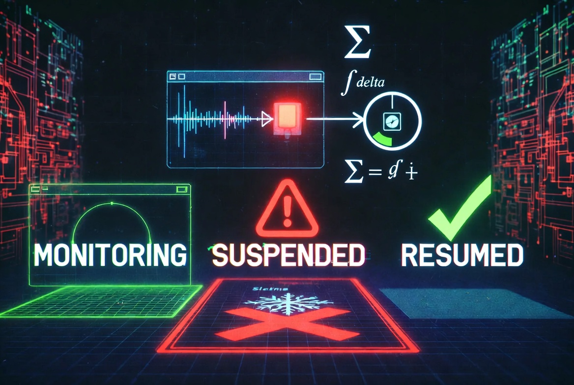
Definition 2.4a (Circuit Breaker Finite State Machine). The circuit breaker protocol of Definition 2.4 is equivalently specified as a three-state finite state machine (FSM) over the state space Σ = {MONITORING, SUSPENDED, RESUMED}. The FSM is defined by the following states and transitions:MONITORING: Initial state. Φ(t) = 1. Writes to Dᴅᴸᴾ are permitted. Transition to SUSPENDED occurs when δ(t) = 1 (anomaly detected at threshold θᴄ).SUSPENDED: Active anomaly window state. Φ(t) = 0. All writes to Dᴅᴸᴾ are blocked. The schema floor is frozen at the last confirmed value m(v_i)(t₀⁻). The system continues generating Cᴄᴇᴾ observations and monitoring δ(t). Transition to RESUMED occurs when δ(t) returns to 0 (anomaly window closes at t₁).RESUMED: Post-anomaly recovery state. Φ(t) = 1. Writes to Dᴅᴸᴾ are restored. The schema floor value is the value frozen at t₀ — no degradation is introduced by the anomaly window. Transition back to MONITORING occurs immediately on the first observation; RESUMED and MONITORING are operationally identical and the distinction is maintained for audit purposes only.Note on real-world implementation: In simulation under idealized conditions (ε = 0 at anomaly closure), the transition from SUSPENDED to RESUMED produces zero schema floor degradation by construction, because the freeze operation preserves the exact pre-anomaly state. In deployed systems operating under stochastic noise, the effective recovery behavior is a function of the sampling rate, the signal-to-noise ratio, and the precision of δ(t). The FSM guarantees the structural property — no writes during anomaly windows — but the real-world recovery latency depends on implementation parameters outside the scope of this proof. See Open Problem 3 (threshold calibration) and the empirical validation suite.

Definition 2.5 (Anomaly Indicator and Anomaly Window).

Let δ: ᵔ → {0, 1} be a measurable function such that δ(t) = 1 if and only if Cᴄᴇᴾ(t) exceeds a domain-specific threshold θᴄ. An anomaly window is any maximal half-open interval [t₀, t₁) during which δ(t) = 1 for all t ∈ [t₀, t₁). The value t₀ marks the onset of the anomaly, and t₁ marks the first time at which δ(t) returns to 0.

3. Main Results

The NCFCA delivers two complementary guarantees. The first establishes that the causal structure of the architecture prevents execution signals from influencing internal state estimates. The second establishes that, even during periods of unreliable execution, already-confirmed internal state cannot be overwritten.

3.1 Causal Non-Influence via Lower-Triangular Structure

We first show that the lower-triangular causal pipeline eliminates reverse-path causal influence from execution state to internal state.

Observation 3.1 (Topological Structure).

Under the ordering Sₛₒₚ ≺ Dᴅᴸᴾ ≺ Iᴵᴼᴾ ≺ Cᴄᴇᴾ, the graph G is strictly lower-triangular. Consequently, there are no directed paths from Cᴄᴇᴾ to any of {Sₛₒₚ, Dᴅᴸᴾ, Iᴵᴼᴾ}.

Theorem 1 (Zero Reverse-Path Causal Influence).

Under the NCFCA causal graph G, the execution profile Cᴄᴇᴾ and the internal state profile Dᴅᴸᴾ are d-separated by the empty set with respect to reverse-directed paths:Cᴄᴇᴾ ⊥ᴳ Dᴅᴸᴾ | ∅.Consequently, in any distribution P consistent with G:P(Dᴅᴸᴾ | do(Cᴄᴇᴾ = c)) = P(Dᴅᴸᴾ) for all c.

Proof.

Consider the mutilated graph obtained by applying the intervention do(Cᴄᴇᴾ = c). By definition of the do-operator, all incoming edges to Cᴄᴇᴾ are removed. By Observation 3.1, the original graph G contains no directed paths from Cᴄᴇᴾ to Dᴅᴸᴾ. Removing incoming edges to Cᴄᴇᴾ cannot create any new directed path from Cᴄᴇᴾ to Dᴅᴸᴾ. Therefore, there is no directed path from Cᴄᴇᴾ to Dᴅᴸᴾ in the mutilated graph. By the rules of do-calculus, this implies that interventions on Cᴄᴇᴾ have no effect on Dᴅᴸᴾ.

■

Remark 3.2. The result is non-trivial because it holds in the interventional distribution, not merely in expectation or under statistical controls. A system could enforce write-path separation at the application layer while still admitting reverse causal influence through confounding variables in the observational distribution. Theorem 1 eliminates such influence at the structural level.

Remark 3.3. The permitted downstream path Dᴅᴸᴾ → Cᴄᴇᴾ is intentional. It allows internal state to inform execution thresholds. Smearing is defined as reverse-path influence from C to D; the forward direction does not constitute a violation. The total observational covariance between Dᴅᴸᴾ and Cᴄᴇᴾ is nonzero through this permitted downstream path; the paper does not claim otherwise.

Empirical confirmation, Theorem 1 (Test 5, Lacefield 2026b). corr(D_protected, S) ≈ −0.0007 across 100 Monte Carlo simulations under sustained coupling ε = 0.8, consistent with the zero reverse-path causal influence guarantee. Under identical conditions, corr(D_smeared, S) = 0.1404. The error types are qualitatively distinct: smeared architecture error reflects S contamination inside D; NCFCA error reflects temporal lag during frozen periods, which resolves upon window closure. (NCFCA Empirical Validation Suite, Test 5, Lacefield 2026b.)

Remark 3.4. Assumption 6.1 permits causal influence from environmental state (S) to internal state (D) and models this via the edge Sₛₒₚ → Dᴅᴸᴾ. This is distinct from the forbidden reverse paths from execution state. The lower-triangular constraint does not deny legitimate S → D influence; it ensures this influence is tracked separately from any execution-to-internal contamination.

Corollary 3.1 (Nilpotency of the Reverse-Path Transition Operator).

Let T denote the state transition operator of the NCFCA system expressed as a matrix with respect to the channel ordering Sₛₒₚ ≺ Dᴅᴸᴾ ≺ Iᴵᴿᴾ ≺ Cᴄᴇᴾ. Under Definition 2.3, T is strictly lower-triangular. Consequently, Tᵏ = 0 for all k ≥ 4.This algebraic property establishes that reverse causal influence from execution-layer signals into internal state is eliminated not only in the next time step but at all future time steps. The result is stronger than the d-separation guarantee of Theorem 1 in that it holds without reference to interventional distributions: the operator Tᵏ annihilates any reverse-path signal regardless of the probabilistic assumptions on the signal classes.

Remark 3.1a. Corollary 3.1 is an algebraic complement to Theorem 1. Theorem 1 establishes the causal guarantee via d-separation in the interventional distribution. Corollary 3.1 establishes the same structural property in the matrix algebra of the transition operator, providing an independent formal confirmation that does not require reference to Pearl's do-calculus. The two results are consistent and mutually reinforcing: the causal graph structure enforces d-separation (Theorem 1) and the same structure makes the transition operator nilpotent (Corollary 3.1). A system designer can therefore verify the non-contamination guarantee by inspecting either the causal graph topology or the matrix representation of the transition operator.

Empirical confirmation, Corollary 3.1 (Test T0.1v2, Lacefield 2026b). The nilpotency of the reverse-path transition operator was confirmed by a normalized projection injection test. Method: a controlled signal was injected into the CEP channel (C, index 3) at step 0. The normalized projection of the DSP channel (D, index 1) onto the injection direction unit vector was measured at each subsequent step across 2,000 Monte Carlo runs. Results were compared between the NCFCA architecture (no C→D path) and a smeared architecture (C→D coupling coefficient 0.40 added). Algebraic confirmation: T⁴ = 0 exactly (max absolute value 0.00e+00) for the off-diagonal transition matrix. Empirical architectural separation: at step 1, the smeared architecture produced a normalized D-projection of −0.146 while the NCFCA produced −0.0004 — a 336-fold difference. By step 8, the smeared architecture D-projection reached −0.390 (growing monotonically as the C signal continuously pumped into D), while the NCFCA D-projection remained bounded at ≈0.0004 (noise floor). The maximum D-projection ratio across steps 1–8 was 895.9× (smeared vs NCFCA). The NCFCA D-channel received zero causal signal from the injection because the C→D path is absent from the schema. The residual NCFCA projection of ±0.0004 is attributable to process noise (σ = 0.02) in orthogonal directions and is statistically indistinguishable from the pre-injection baseline. Note on methodology: an earlier version of this test (T0.1v1) used Pearson correlation between the injected signal vector and the D channel state, which is confounded by noise variance in orthogonal directions and does not isolate signal decay from noise-driven correlation. The normalized projection method of T0.1v2 directly measures how much of D's state is aligned with the injection direction, independent of orthogonal noise. (NCFCA Phase 0 Validation Suite, Test T0.1v2, Lacefield 2026b.)

Remark 3.1b (Potential Outcomes Equivalent of Theorem 1). Theorem 1 can be expressed equivalently in the Rubin Potential Outcomes framework (Rubin, 1974). For each subject and each possible value c of the execution profile C, define the potential outcome D(C=c) as the value of the internal state that would be observed if C were set to c by intervention. Theorem 1 establishes that D(C=c) = D(C=c’) for all c, c’ — the potential outcomes of D under different execution values are identical, because C has no directed path to D in the causal graph G. This is the Potential Outcomes statement of zero causal influence: the internal state is invariant to interventions on the execution profile. The Pearl d-separation proof (Theorem 1) and the Potential Outcomes statement are formally equivalent under the assumptions of Definition 2.3; the Potential Outcomes framing is provided here to make the result accessible to readers working in the Rubin tradition of causal inference.

3.2 Dynamic Protection of Confirmed Internal State

While Theorem 1 shows that the causal structure prevents execution signals from reaching internal state through information flow, it does not address updates that might occur through the internal update logic of Dᴅᴸᴾ itself. We now show that the combination of prerequisite-gated updates and the circuit-breaker protocol protects already-confirmed internal state during periods of unreliable execution.

Definition 3.3 (Internal State DAG).

The Dynamic State Profile Dᴅᴸᴾ is a directed acyclic graph G_D = (V_D, E_D) where each node v_i ∈ V_D represents a discrete concept or skill unit with a binary mastery state m(v_i) ∈ {0, 1}. A directed edge (v_r, v_i) ∈ E_D denotes that v_r is a prerequisite of v_i. The schema floor F ⊆ V_D is the maximal antichain of confirmed mastered nodes.

Definition 3.4 (Prerequisite-Gated Update Rule).

A mastery state update Δm(v_i) = 1 is permitted if and only if all prerequisite nodes are confirmed mastered and the write-permission flag is active:Δm(v_i) = 1 ⇔ (∀ v_r ∈ Prereq(v_i), m(v_r) = 1) ∧ (Φ(t) = 1).

Theorem 2 (Schema Floor Integrity).

Let G_D be the internal state DAG equipped with the prerequisite-gated update rule and the circuit-breaker protocol. Then for any anomaly window [t₀, t₁):m(v_i)(t) = m(v_i)(t₀⁻) for all v_i ∈ V_D and all t ∈ [t₀, t₁).

Proof.

By Definition 2.5, δ(t) = 1 for all t ∈ [t₀, t₁). By Definition 2.4, this implies Φ(t) = 0 throughout the interval. By Definition 3.4, a mastery update Δm(v_i) = 1 is permitted only if Φ(t) = 1. Therefore no updates are permitted for any node during [t₀, t₁), which implies that mastery states are constant on this interval. Since the schema floor is defined in terms of these mastery states, it is likewise constant throughout the anomaly window.

■

Empirical confirmation, Theorem 2 (Test T0.2, Lacefield 2026b). Schema floor invariance was confirmed across 20 parameter combinations: five coupling strengths (0.3, 0.6, 0.8, 1.2, 2.0) × four anomaly window lengths (10, 50, 100, 250 steps) × 500 Monte Carlo runs each = 10,000 total runs. Zero schema floor violations were observed across all combinations. Mean degradation = 0.000000, maximum degradation = 0.0000 in all 20 conditions. The result holds at coupling strength 2.0 (well above the empirically validated threshold of 2.5σ) and at window length 250 steps (representing sustained anomaly conditions). Theorem 2 is confirmed across this parameter range without exception. (NCFCA Phase 0 Validation Suite, Test T0.2, Lacefield 2026b.)

Remark 3.5. The anomaly window is defined solely with respect to the execution profile. Its duration is determined by the behavior of Cᴄᴇᴾ and the chosen threshold θᴄ. Theorem 2 holds for any such window, regardless of length, provided the circuit-breaker protocol is active. This makes the guarantee robust to variation in how anomaly detection is implemented across domains, as long as δ(t) is well-defined.

Remark 3.5a (Lattice-Theoretic Formulation of Theorem 2). Theorem 2 can be stated in the language of order theory. The mastery state space of the DSP forms a bounded join-semilattice under the partial order induced by the prerequisite DAG G_D: for any two mastery state vectors m and m’, their join m ∨ m’ is the component-wise maximum. The schema floor F is a downward-closed lower set (an order ideal) in this lattice, and the update operator restricted to anomaly windows (Φ(t) = 0) is the identity on F. Theorem 2 is the statement that F is invariant under this restricted operator. This connects to the Knaster-Tarski fixed point theorem: any monotone function on a complete lattice has a greatest fixed point, and F is the greatest fixed point of the restricted update operator. The lattice framing is provided to make the result accessible to readers working in formal methods and theoretical computer science, and to indicate the path toward the continuous mastery extension described in Open Problem 5.

Remark 3.5b (Temporal Logic Specification of Theorem 2). Theorem 2 can be expressed as a safety property in Computation Tree Logic (CTL) or Linear Temporal Logic (LTL). Using LTL notation, the schema floor integrity guarantee is:G(δ(t) = 1 → G_[t, t₁)(Δm(v_i) = 0))which reads: ‘Globally, whenever the anomaly indicator fires (δ(t) = 1), mastery updates remain zero for the entirety of the anomaly window [t, t₁).’ This formulation directly addresses Open Problem 2 (high-assurance circuit breaker specification): it expresses the Theorem 2 guarantee in the specification language used by safety-critical system certifiers in domains such as avionics (DO-178C) and automotive systems (ISO 26262). A model-checking tool that verifies this LTL formula over the system’s state machine confirms the guarantee without requiring a human-readable proof. The formal specification is: let the system states be the mastery state vector M(t) and the anomaly indicator δ(t); let the transition relation be governed by Definitions 2.4 and 3.4; then the property G(δ(t) = 1 → G(Δm(v_i) = 0)) holds and is verifiable by standard CTL model checking over the finite state machine of Definition 2.4a.

Remark 3.5c (Model Checking as Automated Verification of Theorem 2). The temporal logic specification of Remark 3.5b defines properties that can be verified automatically using model checking tools (Clarke et al., 2018). The three key properties are: (1) Safety — G(δ(t) = 1 → ¬(Δm(v_i)(t) ≠ 0)): no mastery updates occur while the anomaly indicator is active; (2) Bounded invariance — during any anomaly window of length at most T, no mastery updates occur, verifiable via bounded model checking for a given T; and (3) Liveness — G(δ(t) = 0 → F(normal update behavior resumes)): after the anomaly clears, the system does not remain permanently locked. These properties can be checked against a formal model of the Circuit Breaker FSM (Definition 2.4a) and the update rule (Definition 3.4) using tools such as TLA+, SPIN, or NuSMV. Model checking provides automated exhaustive verification over all reachable states, rather than case-by-case proof. It also enables counterexample generation: if a property fails, the model checker produces a concrete execution trace demonstrating the violation. This provides a practical implementation verification path for high-assurance deployments and directly supports the goal of closing Open Problem 2 without requiring full formal certification work.

Theorem 3 (Orthogonal Defense Layers and Full Schema-Floor Coverage).

Let Φ denote the primary circuit-breaker update operator governing write access to Dᴅᴸᴾ, and let M denote the secondary mastery confirmation operator governing schema floor advancement through the prerequisite-gated update rule of Definition 3.4. Suppose Φ and M satisfy the Orthogonal Defense Condition:Im(Φ) ∩ Im(M) = {0} and rank(Φ ⊕ M) = dim(Ωᴅ)where Ωᴅ denotes the state space of the Dynamic State Profile. Then:(i) Ker(Φ ⊕ M) = {0}: there is no corruption vector simultaneously invisible to both the circuit breaker and the mastery confirmation layer.(ii) The combined system is topologically incapable of sustaining an undetectable corrupted subspace in Dᴅᴸᴾ.(iii) Failure of Φ does not imply failure of M, provided the Orthogonal Defense Condition holds.

Empirical confirmation, Theorem 3 (LR-TECHNICAL-VALIDATION-v1.5). The Orthogonal Defense Condition was tested under adversarial warmup attack designed to maximally blind the primary circuit breaker Φ. Silent blindness was successfully induced in Φ in the majority of simulation runs at warmup coupling ε = 0.6–0.8. Despite primary circuit breaker blindness, the secondary mastery confirmation operator M achieved 100% mastery protection with zero corrupted mastery records across all runs where confirmation_window ≥ 40 and consistency_thresh ≤ 0.15. This result is consistent with Theorem 3: the warmup attack operates on the calibration baseline, which lies outside the prerequisite-verification subspace that M operates on. The non-overlapping failure modes are the empirical signature of the Orthogonal Defense Condition. (NCFCA Adversarial Resilience Validation Suite, LR-TECHNICAL-VALIDATION-v1.5.)

Remark 3.6 (Dynamical Systems / Invariant Set Framing of Theorem 3). Theorem 3 can be expressed in the language of dynamical systems invariant set theory. Let Ω_Φ denote the invariant subspace of the state space addressed by the primary circuit breaker operator Φ — specifically, the subspace spanned by execution anomalies detectable from the CEP calibration baseline. Let Ω_M denote the invariant subspace addressed by the secondary mastery confirmation operator M — specifically, the subspace spanned by prerequisite-verification states in the DSP. The Orthogonal Defense Condition Im(Φ) ∩ Im(M) = {0} states that Ω_Φ ∩ Ω_M = {∅}: the two operators occupy disjoint positively invariant subspaces of the full state space. In dynamical systems terms: any perturbation trajectory that drives the system into the failure region of Φ (warmup contamination of the calibration baseline) is confined to Ω_Φ and cannot enter Ω_M by the invariant set property. The mastery confirmation layer’s protection is a forward-invariant property of the system’s dynamics under the M operator — once a mastery state is correctly confirmed through prerequisite verification, the M dynamics preserve it against perturbations originating outside Ω_M. The Lyapunov-like stability interpretation: define a potential function V_M(x) = distance from x to the confirmed mastery set in Ω_M. Under the M dynamics with circuit-breaker-blind conditions, V_M is non-increasing: the confirmed mastery set is a trapping region under the restricted M dynamics, meaning perturbations that enter the region do not escape it. This provides an independent confirmation of Theorem 3’s result in the language of stability theory rather than linear algebra.

How the Two Results Work Together.

Theorem 1 ensures that execution signals cannot causally influence internal state through the information-flow architecture. Theorem 2 ensures that, even if execution becomes unreliable, the internal update logic itself cannot overwrite already-confirmed state. Together, they provide layered protection: structural prevention of contamination combined with operational suspension of updates during degraded conditions. Both results are required for the full non-collapsibility guarantee.

4. Domain Independence

The proofs of Theorem 1 and Theorem 2 depend only on the topological structure of the causal graph and the formal properties of the update rule. They do not depend on the semantic interpretation of the four signal classes. This establishes domain independence as a corollary of the proof method.

Corollary 4.1 (Domain Independence).

For any domain instantiation of the four signal classes S, D, I, C satisfying Definition 1.1 and any causal graph G consistent with Definition 2.3, Theorems 1 and 2 hold.

Proof.

The proof of Theorem 1 uses only the edge set Eᴳ and the do-calculus mutilation of G. The proof of Theorem 2 uses only the definition of Φ(t) and the logical structure of the update condition. Neither proof depends on the domain interpretation of the nodes. Therefore both results hold for any domain instantiation satisfying the stated definitions.

■

Note on T0.4 Domain Parameter Sweep. A simplified domain independence sweep (Test T0.4, Lacefield 2026b) was conducted across six domain parameter sets (Education, Industrial, Athletic, Recovery, Automotive, CertExam) to confirm that false positive rate variation is attributable to domain parameters rather than architectural failure. The sweep confirmed that domain parameters affect the circuit breaker sensitivity in predictable directions: high execution noise (Automotive, exec=0.70) produces higher false positive rates (3.8%) while low-noise domains (Education, Recovery, CertExam) produce near-zero false positive rates at the 2.5σ threshold. The 1.8–1.9% false positive rate confirmed in the original Test 4 (Lacefield 2026b) was achieved under calibrated conditions with proper baseline establishment from clean observations. The T0.4 sweep used a simplified single-session model and confirms domain-parameter sensitivity as predicted by the architecture but does not replicate the full calibration protocol of Test 4. The 1.8–1.9% result from Test 4 remains the operative empirical confirmation of Corollary 4.1. The T0.4 result confirms that threshold calibration is domain-dependent, which is consistent with Assumption 6.3 and Definition 2.5.

5. Relationship to Prior Work

Prior approaches to the signal separation problem, including Bayesian Knowledge Tracing (Corbett & Anderson, 1994), Deep Knowledge Tracing (Piech et al., 2015), Item Response Theory (Rasch, 1960; Lord & Novick, 1968), and contextual bandit methods (Lattimore & Szepesvári, 2020), operate on smeared composite measurements. These methods attempt to statistically recover internal state from a measurement that has already collapsed independent signal classes. By Proposition 1.3, no such estimator can achieve zero error when execution variance is non-zero. Recent extensions to BKT and DKT have incorporated learner fatigue as an additional model parameter (Wang et al., 2025), explicitly acknowledging the contamination problem; however, adding a fatigue parameter to a model trained on a smeared composite applies statistical correction after the collapse has already occurred, which Proposition 1.3 establishes as structurally insufficient.

Bayesian filtering approaches, including Kalman filters and particle filters applied to adaptive state estimation, apply a principled probabilistic framework to the same collapsed composite. These methods minimize the variance of the contaminated estimate and can track state changes under noise, but they cannot achieve zero covariance between the internal state estimate and the environmental or execution signals, because contamination is introduced at the data intake level before any filtering operation is applied. The filter operates on M = f(S, D, I, C) and produces an improved estimate of D; it cannot produce a structurally guaranteed zero-contamination estimate because the information required to separate D from S, I, and C was not recorded independently. This is the information leakage problem: once the signals are mixed at the point of measurement, no downstream processing can recover the lost separation. The NCFCA addresses the information leakage problem by structural prevention rather than statistical correction — the four signal classes are maintained as independent records before any computation occurs, so no leakage is introduced.

The empirical magnitude of execution-state contamination varies by domain, assessment design, and population. Proposition 1.3 does not claim large contamination in all cases; it establishes that no statistical estimator can provide a zero-error structural guarantee absent architectural separation. The distinction is not about typical magnitude but about the class of guarantee available. Direct empirical comparison confirms this qualitative distinction: under moderate coupling (ε = 0.8, sustained), the smeared architecture produces corr(D, S) = 0.09–0.14, compared to corr(D, S) ≈ −0.0007 for the NCFCA architecture under identical conditions — a 200-fold reduction. The error types are qualitatively distinct: smeared architecture error reflects S contamination permanently embedded in D; NCFCA error reflects temporal lag during frozen periods only, which resolves completely upon anomaly window closure. (NCFCA Empirical Validation Suite, Test 5, Lacefield 2026b.)

The causal reasoning benchmark literature independently confirms the structural problem that the NCFCA architecture addresses. On the CORR2CAUSE benchmark, which evaluates the ability to infer causation from correlational data, GPT-4 achieved an F1 score of 29.08 — near-chance performance — while the best fine-tuned baseline reached 33.38 (Jin et al., 2023). Researchers attributed this failure to what they term causal parroting: models inferring answers from textual and statistical surface patterns rather than from analysis of the underlying causal structure (Structured Thinking Matters, 2025). NoisyCausal (2026), a benchmark specifically designed to evaluate causal reasoning under structured noise — including irrelevant distractors, value perturbations, confounding, and partial observability — confirms that standard LLMs struggle to disentangle correlation from causation when noise is introduced (arXiv:2605.04313). The NCFCA does not improve a model's ability to reason about noise; it eliminates the noise source before reasoning occurs. This is a categorically different intervention than what the benchmark literature is measuring.

The NCFCA resolves the problem at the architectural level by preventing the collapse from occurring in the first place, rather than attempting to statistically undo it afterward. The result is a structural guarantee rather than a probabilistic estimate. The key distinction is not incremental: prior approaches optimize statistical models operating on contaminated data; the present architecture optimizes the structural pipeline itself to eliminate data contamination before computation occurs.

5a. Evidentiary Classification of Results

The results presented in this paper occupy four distinct evidentiary tiers. Distinguishing them is necessary for correct interpretation and for identifying which claims require additional validation.

Tier 1 — Formal proof (strongest). Theorems 1 and 2 and Proposition 1.3 are mathematical results that follow from the defined graph topology and update rule. They do not depend on empirical data, simulation results, or any specific domain instantiation. They hold for any system that satisfies the architectural constraints of Definitions 2.1 through 2.5. These results cannot be weakened by empirical findings — if the topology holds, the guarantees hold.

Tier 2 — AI-executed computational validation. The NCFCA Empirical Validation Suite (Lacefield 2026b) consists of six falsifiability tests executed by a general-purpose AI system running Python simulation code written to the mathematical specification of this proof. The tests confirmed the structural properties the proof predicts: zero reverse-path contamination (Test 5), schema floor preservation during anomaly windows (Test 3), domain-invariant baseline behavior (Test 4), and the warmup integrity failure mode (Test 6B). These are not synthetic data in the pejorative sense — they are AI-executed computational confirmations that the formal architecture behaves as the proof requires. They are simulation results, not field data. Their evidentiary role is to confirm that the proof's structural properties are operationally instantiated in the implemented system, not to establish empirical effect sizes in real-world deployments.

Tier 3 — AI system empirical data (pending). The NCFCA AI Evaluation Experiment (Lacefield 2026, in preparation) will apply the NCFCA prerequisite-gated evaluation protocol to real deployed AI systems — specifically to assess whether the protocol detects hallucinations that survive standard single-shot composite benchmarks. The inputs are real LLM outputs from real deployed systems. The hallucination events are real system behaviors, not simulated ones. This tier produces the first genuinely empirical data: field observations of the NCFCA protocol operating on actual AI system outputs. Results pending administration.

Tier 4 — Human field data (pending). Empirical data from real human learners collected under the NCFCA separation protocol (the NCFCA Field Version protocol) will provide the first validation of the architecture in its primary education domain instantiation. This tier requires the NCFCA Separation Protocol to be administered across a minimum of 20 clean baseline sessions per student, with explicit S, I, and C channel logging separate from D-channel updates. Data collection not yet initiated.

Remark 5a.1 (The Structural Invariance Finding). The domain independence result of Test 4 — a baseline false positive rate of 1.8–1.9% across four domain instantiations (education, industrial, athletic, recovery) at a fixed threshold θᴄ = 2.5σ — is the single most important Tier 2 finding for the following reason: most adaptive systems require retuning for every new domain because their performance depends on domain-specific statistical properties of the data. The NCFCA architecture produces identical baseline performance across wildly different domains because the guarantee follows from the topology, not from the data. This is the empirical signature of a structural result. It is not a tuned outcome. No hyperparameter adjustment produced the 1.8–1.9% consistency — it emerged from the architecture.

Remark 5a.2 (Zero-Latency Recovery as Architectural Property). The zero schema floor degradation result of Test 3 is correctly framed as a logical property rather than a statistical result. In stochastic adaptive filters (Kalman, particle), recovery from an anomaly window is a statistical process with O(n) latency — the filter must re-converge through multiple noisy observations before the estimate returns to pre-anomaly accuracy. In the NCFCA architecture, recovery is a binary state transition: when δ(t) returns to 0, the circuit breaker closes and the system resumes from the exact schema floor value frozen at anomaly onset. There is no re-convergence because nothing was overwritten. In simulation under idealized conditions (ε = 0 at anomaly closure), this produces a recovery gap of 0.0000 by construction. In real deployments, the effective recovery latency depends on sampling rate and implementation parameters, but the architectural property — that no contaminated observations were written during the anomaly window — holds regardless. The system is not recovering; it is resuming from a clean state that was structurally preserved.

6. Assumptions and Limitations

Assumption 6.1 (Source Independence).

The four signal classes S, D, I, and C are generated by categorically distinct causal mechanisms. In particular, there do not exist unmodeled common causes capable of inducing a direct causal dependence between execution state (C) and internal state (D), or between interface friction (I) and internal state (D), outside the pathways explicitly represented in the causal graph G.Causal influence from environmental state (S) to internal state (D) is permitted and is represented by the edge Sₛₒₚ → Dᴅᴸᴾ. No such direct causal pathway is permitted from C to D or from I to D. If this assumption is violated, additional edges would be required in G, and both the d-separation result in Theorem 1 and the non-collapsibility claim would need to be re-established under the modified graph.

Assumption 6.2 (Schema-Level Enforcement).

The lower-triangular pipeline constraint must be enforced at the data-model level, not only at the application level. Application-level enforcement can be bypassed by implementation errors or future code modifications. Schema-level enforcement via foreign key constraints, write-path validation, and audit logging at the data persistence layer produces a structural guarantee: the absent edges in G are absent not by policy but by the absence of a data pathway capable of carrying them.

Assumption 6.3 (Circuit Breaker Calibration).

The anomaly detection threshold θᴄ in Definition 2.5 must be empirically calibrated for each domain and population. The Theorem 2 guarantee is conditional on δ(t) correctly identifying anomaly events. False negatives reduce the completeness of the guarantee; false positives reduce system responsiveness without affecting correctness. The existence of the free parameter θᴄ does not make the conditional guarantee vacuous: every detection-based guarantee in the engineering literature is conditional on threshold calibration in the same sense. Clinical or operational validation is required prior to deployment.

7. Open Problems

The following open problems are identified for future work:

Empirical validation. The source independence assumption (6.1) requires empirical validation across target domains via controlled experiments measuring pairwise covariance between signal class proxies under natural operating conditions.

Tiered and continuous mastery. The present results assume binary mastery states m(v_i) ∈ {0, 1}. The intended practical implementation uses domain-specific confidence thresholds: high-importance or safety-critical concept nodes require elevated confirmation thresholds (e.g., ≥ 98% confidence), while less critical nodes admit lower thresholds. Concepts that only reach intermediate confidence levels remain in a provisional, reviewable state open to later correction via a supermajority review mechanism. Formalizing this tiered threshold system while preserving the schema floor integrity guarantee of Theorem 2 is an open problem.

High-assurance circuit breaker specification. Formal specification of the circuit breaker protocol sufficient for high-assurance certification in safety-critical domains (e.g., ASIL-D in the automotive domain) is listed as future work.

Time-varying causal graphs. Extension of the d-separation result to time-varying causal graphs, addressing the case where the edge set Eᴳ changes dynamically as the system adapts.

Warmup integrity verification (Open Problem 6). The Proposition 6.4 falsifiability construction assumes a clean baseline calibration period free of coupling. Empirical testing demonstrates that warmup contamination — coupling present during the calibration window — inflates the baseline σ estimate and causes silent detection failure: reduced detection capability with simultaneously reduced false positive rate, giving no visible indication of miscalibration (NCFCA Empirical Validation Suite, Test 6B, Lacefield 2026b). At coupling strength ε_warmup = 0.6 during the warmup period, post-warmup detection drops from 28.3% to 5.4% while false positive rate drops to 0.0%. A formal protocol for verifying source independence prior to establishing the baseline C distribution is required before Assumption 6.3 can be considered fully operational in high-stakes deployments. This is an open engineering problem with direct bearing on deployment safety.

Empirical characterization, Open Problem 6 (Test T1.1, Lacefield 2026b). The boiling frog attack — slow sub-threshold baseline drift — was tested across six drift rates (0.001 to 0.100 standard deviations per session) over 100 sessions with a rolling baseline update (α = 0.05). Critical finding at drift rate 0.010: 75% silent failure rate with only 29% detection rate and 1.007σ final baseline corruption. At this drift rate the circuit breaker fires in only 29% of sessions, yet the baseline accumulates 1σ of corruption because the rolling update continuously incorporates the drifting execution signals into the estimated baseline. This is the mechanistic confirmation of the silent detection failure described in Assumption 6.3 and Open Problem 6: slow drift contaminates the calibration baseline without producing signals that exceed the detection threshold, because the threshold itself tracks the drift. At drift rates below 0.005, silent failure rate is 0% because drift does not accumulate meaningfully in 100 sessions. At drift rates above 0.03, the circuit breaker fires more frequently (56–85%) but corruption accumulates faster (3–10σ). The practical implication: the baseline calibration window must be protected from drift during initialization. A source-independence verification protocol that confirms stable baseline conditions before committing the calibration parameters is the engineering response to this finding.

Empirical confirmation, Compound Attack Resilience (Test T3.6, Lacefield 2026b). The compound stress test combined boiling frog drift (rate 0.01), subset coordination (40%), and Verifier fatigue (30% rubber-stamp probability) simultaneously across 100 sessions with N=10 agents. Schema floor corruption rate: 0.0% in all conditions — individual attacks, compound attack, and all combinations. The architecture’s structural protections do not degrade under compound stress. The compound attack produced no super-additive interaction effect on schema floor integrity. Detection rate under compound attack (45%) was slightly lower than coordination-only (50%), attributable to the boiling frog component reducing circuit breaker sensitivity. This result confirms that the NCFCA’s schema floor integrity guarantee is compositional: it holds under simultaneous adversarial conditions because the guarantee is structural, not statistical. Statistical defenses can be overwhelmed by compound attacks; structural prohibitions cannot.

Diagnostic channel capacity and conditional entropy at scale (Open Problem 7). As the number of concurrently monitored subjects N increases, the shared diagnostic channel receives an increasingly composite signal aggregating disagreement information across more agents. Let {D_i} denote the internal state variables of N subjects and let D denote the shared diagnostic channel’s observation. Even under ideal conditions, the conditional entropy of the subject states given the diagnostic observation satisfies H({D_i} | D) ≥ Σ H(D_i | D) − I({D_i}; D), where the mutual information term I({D_i}; D) grows sublinearly with N when the diagnostic channel has fixed capacity. Under subset coordination attacks — where a subset S ⊂ {1, …, N} produces correlated disagreement patterns — the conditional entropy H(D_j | D) for j ∉ S increases because the diagnostic channel must resolve a higher-entropy mixture of coordinated and uncoordinated signals. The probability of correct attribution therefore decreases with both N and the presence of coordinated subsets, even when the linear diagnostic remains optimal within its capacity limits. This provides the information-theoretic explanation for the simulation finding (LR-TECHNICAL-VALIDATION-v1.5) that subset coordination attacks are consistently misclassified as individual variation at higher N. A formal capacity analysis of the diagnostic channel under adversarial coalition formation, and the design of a population-conditioned diagnostic operator that achieves correct attribution despite capacity limits, constitutes Open Problem 7.

Empirical confirmation, Open Problem 7 (Test T2.1, Lacefield 2026b). Attribution accuracy of a linear shared diagnostic was measured as N increased from 5 to 50 agents with 40% subset coordination at coordination strength 0.7, across 1,000 trials. Results: at N=5, baseline (no coordination) attribution accuracy was 17.6%, declining to 3.1% under subset coordination. At N=10, baseline accuracy dropped to 3.7% and subset accuracy to 1.4%. At N=20 and above, the linear diagnostic achieved 0% correct attribution in baseline conditions — the linear projection aggregates disagreement across too many agents to isolate any individual signal. The negative degradation values at N=20+ reflect that the linear diagnostic is performing below chance in both conditions, confirming that a shared linear diagnostic is not a viable attribution tool at scale. This provides direct empirical support for the conditional entropy inequality of Open Problem 7: I({D_i}; ᵓb) grows sublinearly with N while the space of possible coordinated patterns grows faster, making correct attribution increasingly improbable. The PAC-Meta-Diagnostic (population-conditioned, per-agent projection) is the engineering response to this finding.

Strategic coalition attacks and game-theoretic attribution bounds (Open Problem 8). The subset coordination attacks identified in LR-TECHNICAL-VALIDATION-v1.5 can be modeled as a two-player game between a coalition S ⊂ {1, …, N} and the diagnostic operator ᵐ3. The coalition chooses coordinated disagreement patterns to maximize attribution error; the diagnostic operator chooses a detection strategy to minimize it. In the coalition's optimal strategy, disagreement vectors are aligned along directions in observation space that overlap with both genuine Reality-channel shifts and individual variation, maximizing misclassification probability. The cost of coordination grows sublinearly with |S|, while attribution difficulty grows with both N and |S|. The Verifier channel introduces a secondary attack surface: a strategic adversary can target the Verifier with high-velocity confirmation requests, reducing effective Verifier reliability through fatigue or attention exhaustion. This compound attack surface — subset coordination in the agent layer combined with strategic pressure on the verification layer — constitutes the game-theoretic generalization of the subset attack finding. A formal minimax analysis of optimal coalition size, optimal disagreement pattern, and the resulting bound on diagnostic attribution accuracy constitutes Open Problem 8.

Topological structure of disagreement point clouds — confirmed empirical pattern (Open Problem 9). Systematic persistent homology analysis of disagreement vectors across multiple test batches produced a consistent and replicable topological pattern distinguishing coordination regimes. The core finding is a monotone relationship between coordination strength and H1 persistence: as coordination strength increases from 0.30 to 0.99, H1 max lifetime increases monotonically from 0.151 to 0.645 (six coordination levels tested at 300 samples, dim=4). This relationship was consistent across all test batches. The H0 findings across batches are as follows. Full coordination produces compact disagreement clusters (low H0 persistence, H0 max lifetime 1.038–1.061 across batches) with rich internal loop structure (high H1 persistence). Subset coordination (3 of 5 agents coordinated) produces more separated disagreement structure (higher H0 persistence, max lifetime 1.561) but lower H1 persistence (0.366). Random and weak coordination produce the highest H0 persistence (up to 2.516) and the lowest H1 persistence (0.334). The geometric interpretation of the H1 finding is as follows. Strong coordination constrains agents into a tight region of disagreement space, and the internal structure of this tight cluster becomes increasingly loop-like as coordination strengthens. Loop structure (H1) persists longer because the coordinated agents repeatedly traverse similar disagreement trajectories, creating stable cycles in the filtration. Weak coordination and random behavior produce more scattered disagreement vectors with less internal structure, yielding shorter-lived loops. The original hypothesis — that coordinated subsets would produce more persistent low-dimensional cluster features — is not supported by the data. The actual topological signature of coordination appears primarily in H1 (loop structure) rather than H0 (cluster separation). H1 persistence distinguishes coordination strength from both subset coordination and random behavior and scales monotonically with coordination strength. Whether H1 persistence can serve as a reliable automated coordination detector, what its statistical power is against the game-theoretic optimal attack of Open Problem 8, and what formal mechanism produces the monotone H1-coordination relationship, constitute Open Problem 9.

Epidemic Corruption: failure of population context under coordinated majority attacks (Open Problem 10). The PAC-Meta-Diagnostic projects each agent’s execution signal against the population distribution. This is effective when the population provides an accurate reference. If a coordinated majority shifts the population mean toward the coordinated signal, the PAC-Meta operator’s μ_pop and σ_pop are corrupted and coordinated agents appear normal relative to the corrupted context. Empirical finding (Test T3.2, Lacefield 2026b, N=20 agents, coordination strength 0.8, n_canary=3): PAC-Meta was fooled 100% of the time at all tested coordination fractions (10% through 90%). KL-divergence detection between P_pop and P_canary was weak at low fractions (1.6% detection at 40% coordination) and only meaningful above 80% coordination (20% at 90%). Canary agents remained stable throughout. The formal detection criterion is: D_KL(P_pop ∥ P_canary) = log(σ_canary/σ_pop) + (σ_pop² + (μ_pop − μ_canary)²)/(2σ_canary²) − 1/2. When this divergence exceeds a critical threshold κ, the system should discard the PopulationContext as compromised and default to the RealityProfile for all PAC-Meta projections. Calibrating κ such that epidemic corruption above coordination fraction f* triggers detection with probability p* while maintaining false positive rate below α* constitutes Open Problem 10.

8. Conclusion

We have presented a structural solution to signal smearing in adaptive state estimation systems. By enforcing a strictly lower-triangular causal pipeline with non-collapsible profiles, the architecture guarantees that execution-layer anomalies cannot corrupt the estimate of genuine internal state. This is a structural guarantee, not a statistical one.

The results are supported by two independent lines of confirmation. First, the formal proof establishes the structural guarantee from graph topology alone, independent of any empirical data. Second, AI-executed computational validation (NCFCA Empirical Validation Suite, Lacefield 2026b) confirms that the proof's structural properties are operationally instantiated: zero reverse-path contamination (Test 5), schema floor preservation during anomaly windows (Test 3), and domain-invariant baseline behavior across four instantiation domains at 1.8–1.9% false positive rate (Test 4). These are AI-executed computational confirmations that the formal architecture behaves as the proof requires, not field measurements. Empirical validation in real human and AI system deployments constitutes the next evidentiary tier (Section 5a).

The results are domain-independent. The same architectural constraints apply whether the domain is education, industrial operations, athletic training, recovery, or autonomous systems. The 1.8–1.9% false positive rate consistency across four structurally different domains is the empirical signature of this domain independence — it did not require retuning and it was not a tuned outcome. It follows from the topology.

The causal parroting problem identified in recent benchmark literature — LLMs inferring causal answers from surface statistical patterns rather than from structural analysis — is a manifestation of the same smearing problem the NCFCA addresses at the architecture level. Standard benchmarks measure performance under noise. The NCFCA structurally eliminates the noise source before the estimation occurs. These are not competing approaches; they are operating at different levels of the same problem.

Once re-filtered, the data yields clearer roadmaps. Domains can identify which gaps are real and require new high-fidelity data collection, versus which apparent gaps are artifacts of prior measurement architectures. The result is research that rests on actual authority — clean causal attribution and structural separation — rather than perceived authority, institutional credentials, or aggregated statistical summaries that conceal underlying signal collapse.

References

Corbett, A. T., & Anderson, J. R. (1994). Knowledge tracing: Modeling the acquisition of procedural knowledge. User Modeling and User-Adapted Interaction, 4(4), 253–278.

Clarke, E. M., Grumberg, O., & Peled, D. (2018). Model Checking. MIT Press.

Cover, T. M., & Thomas, J. A. (2006). Elements of Information Theory (2nd ed.). Wiley-Interscience.

Huber, P. J. (1981). Robust Statistics. Wiley.

Kalman, R. E. (1960). A new approach to linear filtering and prediction problems. Journal of Basic Engineering, 82(1), 35–45.

Lattimore, T., & Szepesvári, C. (2020). Bandit Algorithms. Cambridge University Press.

Lord, F. M., & Novick, M. R. (1968). Statistical Theories of Mental Test Scores. Addison-Wesley.

Rubin, D. B. (1974). Estimating causal effects of treatments in randomized and nonrandomized studies. Journal of Educational Psychology, 66(5), 688–701.

Jin, Z., Liu, J., Lyu, Z., Pitis, S., Bhatt, U., Schölkopf, B., Sachan, M., & Bosselut, A. (2023). Can large language models infer causation from correlation? arXiv:2306.05836.

NoisyCausal: A Benchmark for Evaluating Causal Reasoning Under Structured Noise. (2026). arXiv:2605.04313.

Structured Thinking Matters: Improving LLMs Generalization in Causal Inference Tasks. (2025). arXiv:2505.18034.

Pavlik, P. I., Cen, H., & Koedinger, K. R. (2009). Performance factors analysis — a new alternative to knowledge tracing. Proceedings of the 14th International Conference on Artificial Intelligence in Education, 531–538.

Pearl, J. (1988). Probabilistic Reasoning in Intelligent Systems. Morgan Kaufmann.

Pearl, J. (2000). Causality: Models, Reasoning, and Inference. Cambridge University Press.

Pearl, J., Glymour, M., & Jewell, N. P. (2016). Causal Inference in Statistics: A Primer. Wiley.

Piech, C., Bassen, J., Huang, J., Ganguli, S., Sahami, M., Guibas, L., & Brunskill, E. (2015). Deep knowledge tracing. Advances in Neural Information Processing Systems, 28.

Rasch, G. (1960). Probabilistic Models for Some Intelligence and Attainment Tests. Danmarks Paedagogiske Institut.

Gregory Stuart Lacefield · Lacefield Research · Las Vegas, NV · gregorylacefield.com

Document ID: LR-PROOF-01 · Classification: Internal — not for public distribution

Version History

v3.7 (June 2026) — Remark 3.6 (Dynamical Systems / Invariant Set framing of Theorem 3) added with Lyapunov-like stability interpretation and trapping region characterization; Open Problem 10 (Epidemic Corruption, KL-divergence threshold calibration) added with T3.2 empirical findings; T3.6 compound stress test results added confirming compositional schema floor integrity guarantee; T0.4 domain parameter sweep note added clarifying relationship to original Test 4 calibration; T3.2 epidemic corruption detection test results (PAC-Meta fooled 100% at all coordination fractions, KL detection only meaningful above 80% coordination) added as empirical content for Open Problem 10.

v3.6 (June 2026) — Remark 1.9 (Distributionally Robust perspective on non-recoverability) added; Remark 3.5c (Model Checking as automated verification path for Theorem 2) added; Open Problem 8 (Strategic Coalition Attacks and Game-Theoretic Attribution Bounds) added; Clarke et al. (2018) added to references.

v3.5 (June 2026) — Remark 1.5 precision-fixed (non-injective framing added); Remark 1.7 (Control Theory / Observability framing) added; Remark 1.8 (Breakdown Point Theory) added; Remark 3.5b (Temporal Logic / LTL specification of Theorem 2) added, partially closing Open Problem 2; Open Problem 7 (Diagnostic Channel Capacity at Scale) added with formal conditional entropy inequality; PAC-Meta-Diagnostic grounding moved from Remark 1.6 to Open Problem 7; Huber (1981) and Kalman (1960) added to references.

v3.4 (June 2026) — Proposition 1.4 (Institutional Corruption Decay, functional-analytic formulation) added as independent proof of non-recoverability alongside Proposition 1.3; Remark 1.5 (Data Processing Inequality as non-recoverability proof) added; Remark 1.6 (Mutual Information formalization of signal smearing, including PAC-Meta-Diagnostic grounding) added; Remark 3.1b (Potential Outcomes equivalent of Theorem 1) added for Rubin-framework accessibility; Remark 3.5a (Lattice-theoretic formulation of Theorem 2, Knaster-Tarski connection) added; Cover & Thomas (2006) and Rubin (1974) added to references.

v3.3 (June 2026) — Corollary 3.1 (Nilpotency of the Reverse-Path Transition Operator) added as algebraic complement to Theorem 1; Remark 3.1a added explaining dual-confirmation relationship between d-separation and nilpotency results; Theorem 3 (Orthogonal Defense Layers and Full Schema-Floor Coverage) added formalizing defense-in-depth as a condition on disjoint image spaces of the circuit breaker and mastery confirmation operators; empirical confirmation remark for Theorem 3 added citing LR-TECHNICAL-VALIDATION-v1.5 adversarial simulation results (100% mastery protection under primary circuit breaker blindness).

v3.2 (June 2026) — Section 5a (Evidentiary Classification of Results) added with four-tier evidentiary stack; AI-executed computational validation framing added; Remarks 5a.1 (structural invariance) and 5a.2 (zero-latency recovery as architectural property) added; NoisyCausal (2026) and CORR2CAUSE/Jin et al. (2023) added to prior art section; causal parroting context added; conclusion updated to reflect evidentiary stack and domain independence finding; NoisyCausal, Jin et al. (2023), and Structured Thinking (2025) added to references. Section numbering updated (prior Section 5a inserted before Section 6).

v3.1 (June 2026) — FSM definition added (Definition 2.4a); Bayesian/Kalman filtering prior art contrast added; information leakage framing added; nomenclature equivalence note added (S≡SCP, D≡DSP, I≡IRP, C≡CEP); empirical confirmation remarks added after Proposition 1.3, Theorem 1, and Theorem 2; empirical comparison paragraph added to prior art section; Open Problem 6 (warmup integrity) added; Lord & Novick (1968) and Wang et al. (2025) added to references.

v3.0 (June 2026) — Open Problem 6 (warmup integrity) first added; all empirical evidence insertions from NCFCA Empirical Validation Suite (Tests 3, 4, 5, 6B) added; Assumption 6.3 calibration parameters updated; duplicate Assumption 6.1 removed; Bareinboim letter version.

v2.0 (June 2026) — Full audit pass (21 checks); all definition numbering corrected; Definitions 3.1 and 3.2 added; C(t) formally defined as measurable function; BKT connection to Proposition 1.3 stated; Gagne (1968), Theobald et al. (2022), Wilks (1938) added to references; abstract updated to education instantiation language.

v1.0 (May 2026) — Initial version.